
In their 2013 report, Mark Jacobson outlined several claims regarding the conversion New York State infrastructure to 100% WWS by 2030. In evaluating the feasibility of their claims with regards to economics, we will investigate the following claims:
- Cost of different energy sources
- Total Job creation and earnings
- Solar
- Wind
- Cost reduction from reduced pollution related mortality and morbidity
______________________________
Introduction
The following discussion covers claims made by Jacobson and associates regarding the current and long term predictions of energy costs. All costs are in 2007 US. Cents/kWh. The primary claim made regarding these data points is that WWS (Wind, Water and Solar) energy sources will trend downward as conventional energy trends upwards. They support this claim with citation of numerous energy studies which predict both current and future energy cost trends.
Within this section the evidence for all claims presented is given in the form of three tables. These tables will each be analyzed individually, and their contents are summarized below.
Table 3: Fully annualized generation and short-term transmission costs for WWS power.
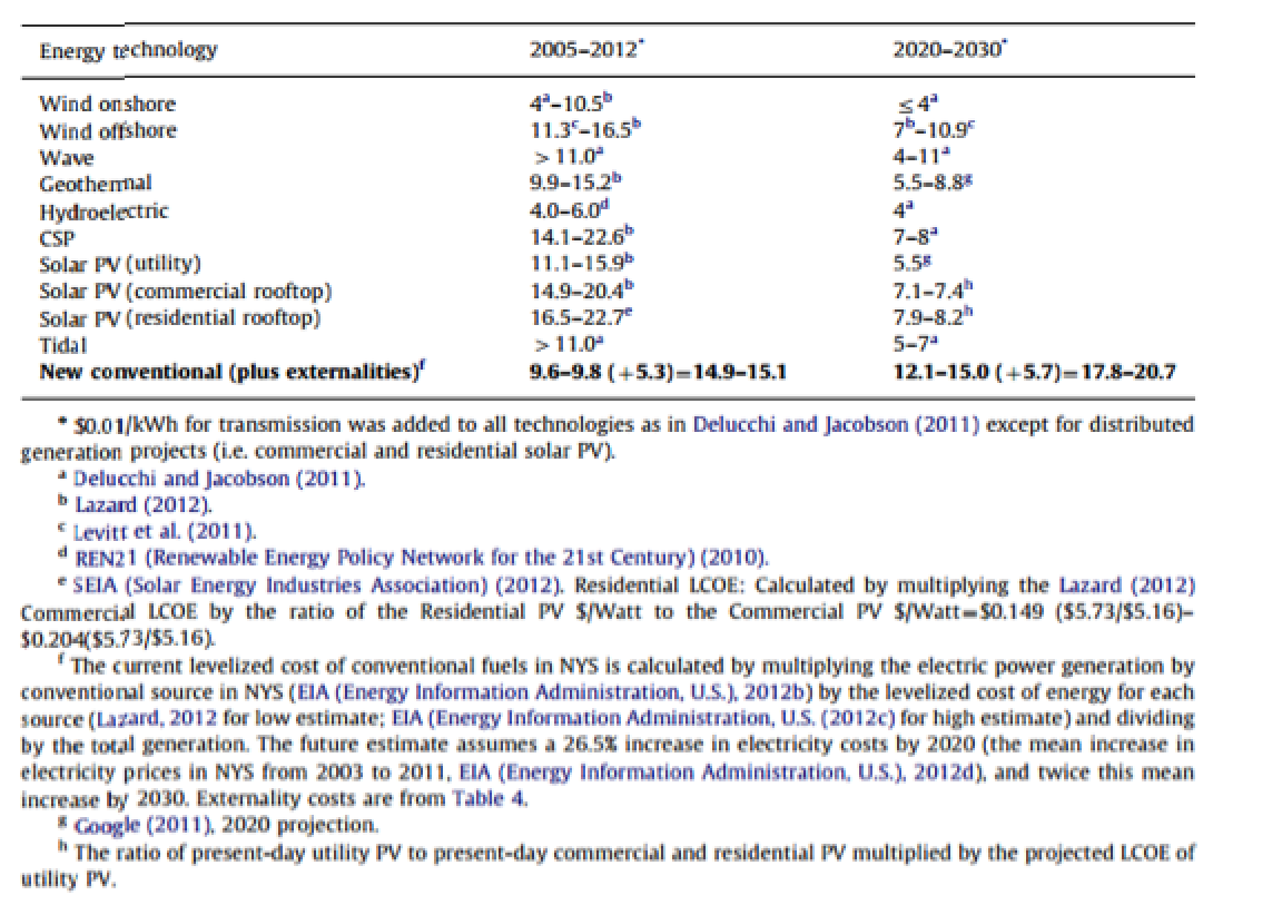
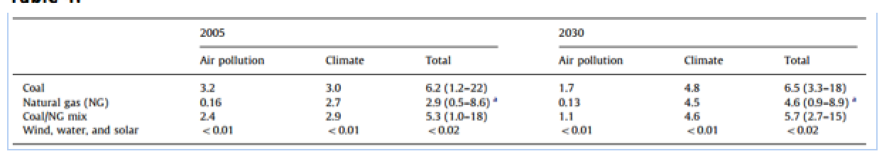
Table 4: Mean & Range of environmental externality costs of coal, natural gas and renewables in the US
Table 5: Projected unit costs of selected conventional fossil fuels over the period 2009-2030 in NYS
Source: Jacobson et al. (2012)
Table 3: Fully annualized generation and transmission costs (Jacobson Et Al. 2013)
Source: Jacobson et al. (2012)
Table 3, taken from the study, describes the current and projected cost of WWS over the next 20 years (in 2007 dollars). These claims are individually analyzed below. Each claim has been analyzed individually based on the cited sources used in the study (See above)
Transmission
For this study, transmission costs were treated individually and then added on to the LCOE estimates. In accordance with Delucchi & Jacobson (2011), a cost of 0.01 $/kWh was added to all generation estimates with the exception of distributed generation projects (commercial and residential. All values presented below are discussed prior to the addition of transmission costs.
Google (2011) provides different transmission estimates, citing approximately transmission costs of 0.05/ 0.10 $/kWh, notably higher then Jacobson. Both studies make the primary assumption that all transmission networks will be implemented prior to 2030. This is a bold claim because it assumes sufficient resources are focused by implementing organizations to complete transition by this time. While this is a generally accepted assumption, failure to implement to this level will lead to increasing inaccuracies in the estimates.
The revised energy cost table we have developed in order to improve feasibility is shown below.
| Energy Technology | 2005-2012 | 2020 – 2030 |
| Wind onshore | 4 – 9.1 | <4 |
| Wind offshore | 11.3 – 22.6 | |
| Wave | > 11.0 | 11-Apr |
| Geothermal | 9.9 – 15.2 | 5.5 -8.8 |
| Hydroelectric | 4.0 – 6.0 | 4 |
| Concentrated Solar Power | 12.8 – 14.0 | < 7 – 8 |
| Solar PV ( Utility) | 8.2 – 9.6 | 5.5 |
| Solar PV ( commercial rooftop) | 13.6 – 18.7 | 7.1 -7.4 |
| Solar PV ( residential rooftop) | 16.5 – 22.7 | 7.9 – 8.2 |
| Tidal | > 11.0 | 5.0 -7.0 |
| New Conventional ( plus externalities) | 14.9 – 15.1 | 17.8 – 20.7 |
(All Values 2007 US $/kWh)
The following discussion covers the sources and feasibility issues with each prediction, and illustrates the process used to arrive at these revised values.
Claim Analysis By Energy Type
(All values in 2007 US $/kWH)
( O&M : Operations & Maintenance)
Onshore Wind Cost
Claim: current onshore wind costs per kWh are 4 – 10.5.
The Lower bound was drawn from Delucchi & Jacobson (2011). The bound was calculated by averaging marginal levelized cost. The range is driven by variations in facility types, scale, and varying capital and operating costs.
The upper bound was drawn from Lazard. Lazard predicts a total of 9.5 cents (before transmission costs) which includes: 7.4 capital costs, 1.1 fixed O&M and 1.0 for variable O&M. This bound is now out dated. To improve the feasibility of this prediction a revised estimate of 8.1 is more accurate. This value includes 6.6 capital costs and 1.5 Fixed O&M costs
Claim: Projected onshore wind costs will be < 4.
Values are drawn from Schilling and Esmundo (2009). This value is supported by similar claims, including Berry’s (2009) and De Carolis & Keith’s (2006).
Off Shore Wind Cost
Claim: current offshore wind costs are 11.3-16.5
Lower bound is drawn from Levitt et al. (2011)
Upper bound is drawn from Lazard (See below for applicable assumptions). When updated based on more recent values (2014), Lazard predicts 21.6, which includes 18.6 capital costs, 2.7 fixed O&M and 3 Variable O&M
Claim: projected offshore wind costs will be 7-10.9
Lower bound is drawn from Lazard (2008). Accuracy can be improved by updating values to reflect 2014 predictions. This improves the estimate to 16.2.
Wave
Claim: Current wave costs are > 11.0
Claim: Projected wave costs will be 4-11
These values are predicted in Delucchi & Jacobson (2011), who cite Bedard et al. (2005). In that study, levelized production was estimated at 0.10 %/kWh for the first plant. Cost was then projected as a function of installed generation capacity using a “learning-curve” model and estimates comparable to wind production.
The primary issue with this approach lies in the comparison between wave and wind. This comparison is itself inaccurate because wind trends are also predictions themselves. In addition, all estimates assume continued development of capital infrastructure. For these reasons this prediction is feasible only for the narrow band of implementation strategy described within the study.
Geothermal
Claim: Current Geothermal costs are 9.9 -15.2
Both upper and lower bounds are taken from Lazard (See below for assumptions). Lower bound includes 5.9 capital costs and 3.0 variable O&M . Upper bound includes 10.2 capital costs and 4.0 variable O&M.
These values have not changed over the period of 2012- 2014. For this reason, we should regard these as feasible predictions of current trends.
Claim: Projected Geothermal costs are 5.5-8.8
These values are predicted by Google (2011) (pg. 4).
Hydroelectric
Claim: Current Hydroelectric costs 4.0 -6.0
Current Hydroelectric cost claims come from REN 21 (2010
Claim: Projected Hydroelectric costs are 4.0
This prediction is drawn from Delucchi & Jacobson (2011).
CSP (Concentrated Solar Power)
Claim: Current CSP 14.1-22.6
Both upper and lower bounds are taken from Lazard. Lower bound includes 11.5 capital costs, 1.3 fixed O&M and .3 variable O&M. Upper Bound Includes 18.6 capital costs, 2.7 fixed O&M and .3 variable O&M.bb
These numbers are now outdated. Feasibility can be improved by updating these numbers to 2014 values. The Lower bound should be revised to 11.8, which includes 10.2 capital costs and 1.6 fixed O&M. The upper bound should be revised to 13.0, which includes 11.2 capital costs and 1.8 fixed O&M.
Claim: Projected CSP costs 7-8
This prediction is taken from Delucchi & Jacobson (2011). This claim predicts a major downward trend in the cost of CSP generation. The feasibility of this claim is based on the developments that occur with this technology along with the assumed increase in pace of development.
Solar PV (Utility)
Claim: Current Solar PV (Utility) 11.1 -15.9
Both Upper and lower bounds are taken from Lazard. Lower bound includes 9.2 capital costs and .9 fixed O&M. Upper bound includes 13.8 capital costs and 1.1 fixed O&M.
These values are outdated. Accuracy of claims is improved through updating these values to reflect 2014 levels. The Lower bound should be changed to 7.2, which includes 6.5 capital costs and .8 fixed O&M. The Upper bound should be changed to 8.6, which includes 7.9 capital costs and .7 fixed O&M.
Claim: Projected Solar PV (Utility) 5.5
This value is taken from Google (2011).
Solar PV (Commercial)
Claim: Current Solar PV (Commercial Rooftop) 14.9 – 20.4
Both of these bounds were taken from Lazard. The lower bound includes 14.3 capital costs and .6 fixed O&M. The Upper bound includes 19.2 capital costs and 1.2 fixed O&M.
These values are outdated. Accuracy of this claim can be improved by updating these values to 2014 levels. The Lower bound should be changed to 12.6, which includes 11.9 capital costs and .6 fixed O&M. The Upper bound should be changed to 17.7, which includes 16.5 capital costs and 1.1 fixed O&M.
Claim: Projected Solar PV (Commercial Rooftop) 7.1-7.4
Solar PV (Residential)
Claim: Current Solar PV (Residential Rooftop) 16.5-22.7
Claim: Projected Solar PV (Residential Rooftop) 7.9-8.2
These values were taken from Lazard (2012), and modified based on the prediction rates for both commercial and residential multiplied by utility rates. These values will suffer from inaccuracies in previous measurements as a result.
Tidal
Claim: Current Tidal > 11.0
Claim: Projected Tidal 5.0-7.0
These values are taken from Delucchi & Jacobson (2011). Primary accuracy problems in this field deal with the relatively few number of tidal facilities that have been constructed in the US. As more facilities come on line, these predictions will improve.
Conventional Fuels (plus externalities)
Claim: Current Conventional 14.9 – 15.1
Claim: Projected Conventional 17.8-20.7
These values are the Levelized Cost of Energy for conventional fuel sources. Methods used for their derivation (Jacobson et al. 2012) are consistent with LCOE models. The increase to both current and projected costs caused by externalities (5.3, 5.7) serves as a framework. However, error will exist in these predictions both at present and over the next 20 years.
Assessment
In addition to the age of data and issues of cited information, There are also a couple larger scale data issues, given below.
- This assumes that large scale transition will occur, which will affect prices
- Levelized cost does not take into account additional fees accrued over the lifetime of the equipment, such as repairs, upgrades, and renovations
Many of the estimates provided are also conflicted by other sources, including the EIA forecast for 2040 (EIA 2014) . These predictions are shown below. When compared, the EIA tends to predict higher LCOE for current construction by 2040 then Jacobson. This trend would suggest that capital costs have increased over the last 5 years in pace with the rate of technological improvement.
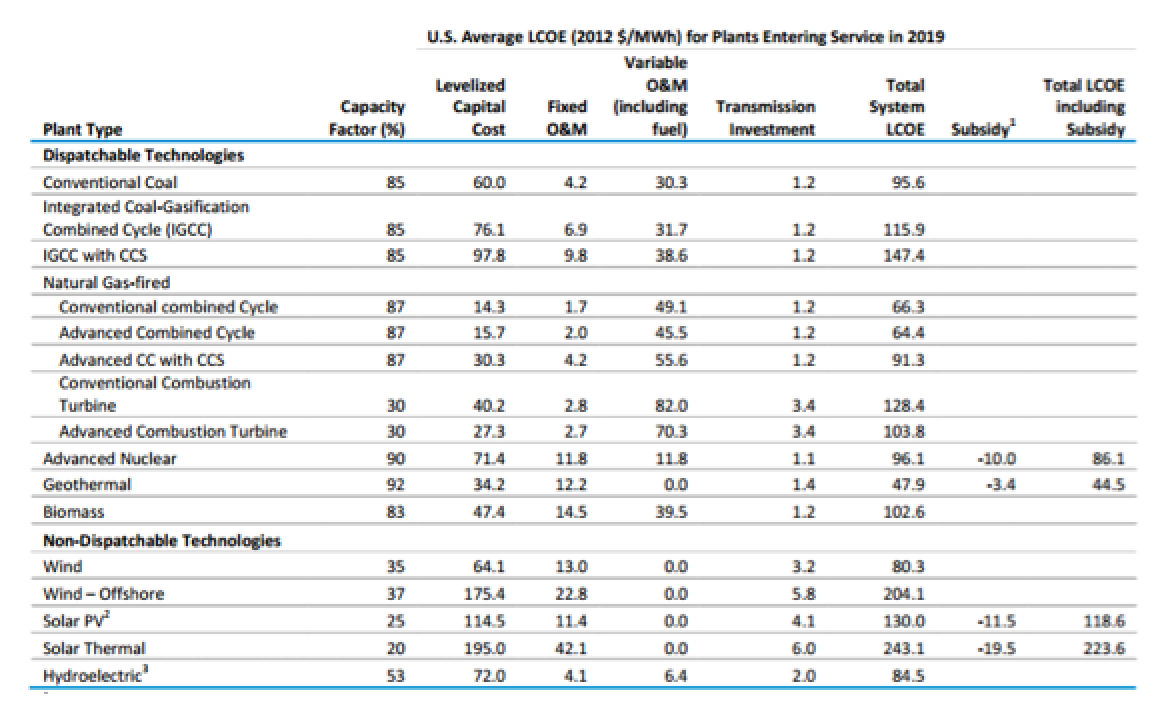
Source: EIA (2014)
Despite these problems, this data still provides a very effective starting point for developing a framework of metrics for predicting and working around energy costs over the next 20 years. The Trends predicted within this study are also supported by the U.S. Energy Information Association).
Environmental Externality Costs
Table 4:
Source: Jacobson et al. (2012)
This table illustrates the predicted environmental externality costs of conventional fuel resources. These values were taken from Delucchi and Jacobson (2011), but modified for mean shale and conventional natural gas carbon equivalent emissions from Howarth et al 2011. In addition, the following fuel mixtures used for energy generation were assumed:
- Shale : Conventional Natural Gas
- 30:70 – 2011
- 50:50 – 2030
- Coal: Natural Gas
- 73:27 – 2005
- 60:40 – 2030
In order to account for the hybrid nature of the conventional fuel supplies showed above, fuels where converted into over all carbon emissions using the concept of Equivalent Carbon Emissions. This calculation provides an estimate for carbon based emissions from ferrous fuel sources.
Delucchi and Jacobson (2011) cite the following values, which have not been modified to account for carbon equivalent emissions.
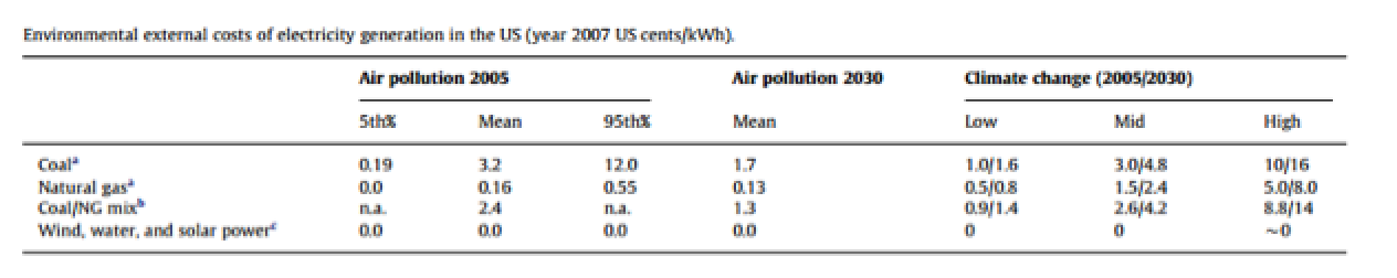
Source: Delucchi & Jacobson (2011)
Assessment
These values reflect an accurate description of conventionally excepted externality values. Primary issues come from the realities of these studies. While the physical energy producing processes of these systems emit no harmful exhaust substances, the overall energy system still poses human risks, which cannot be effectively modeled. These include risks in the capital construction processes. In addition, the nature of environmental externality assessment is inherently inaccurate. The operation of relating environmental damages to human health problems will always have error because of the enormous number of factors involved in the human interaction with environmentally related illnesses.
Cost of Conventional Fuels
Table 5:
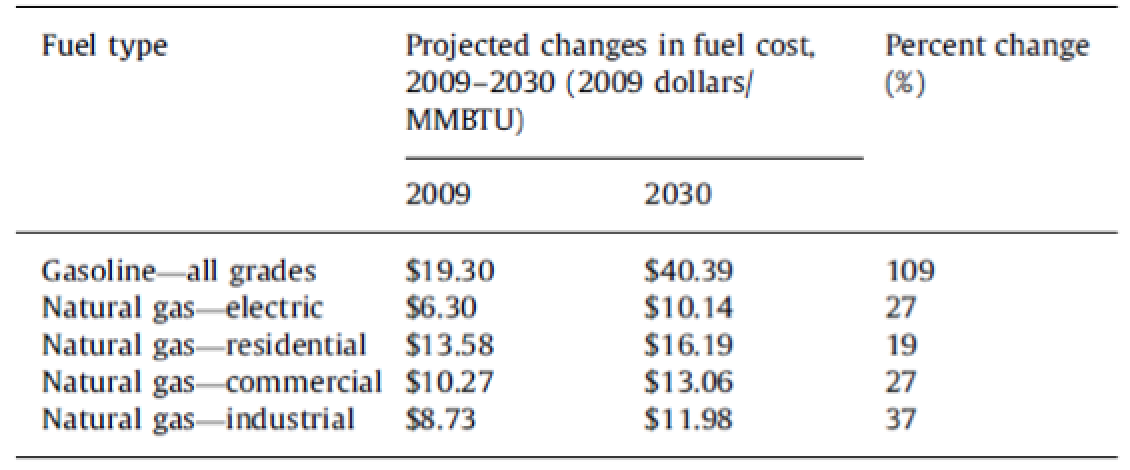
Source: Jacobson et al. 2012
This chart is taken from the New York State Energy Planning Board’s 2009 Energy plan. The study was conducted using the statistical analysis method of Ordinary Least Squares. This method has embedded within it a series of assumptions, listed below.
Experimental data extends back 17 years, using 2007 as a baseline. Primary data sources are listed below.
- NYSERDA Patterns & Trends
- EIA Annual Energy Outlook
- EEA inc. Gas Market Compass
A series of assumptions about existing variables were taken. The following variables were not included within the study
- Peak Oil
- Global Political and Civil Unrest,
- Natural disasters
These variables were considered too complex to be effectively modeled. Unfortunately, these also constitute some of the primary factors effecting global resource prices. For example, OPEC still continues to play a major role in setting oil prices, and they are in large part responsible for the fluctuations we currently experience. OPEC is actually predicting that oil prices will stay low over the next 15-20 years ( below 100$ a barrel). They intend to take action against this ( WSJ, 2015). This situation is made more difficult by the fact that many OPEC nations rely on high oil prices for fiscal solvency. This will lead to a situation where prices are not only fluctuating based on supply and demand, but geo-political realities.
The prices themselves were determined using the Average Annual West Texas Intermediate oil and Henry Hub gas spot prices. The WTI price forecast was developed by NYSEPB using 2 methods
- Delphi Process
- Global econometric oil model developed by ICF International
Assessment
The statistical modeling used in this study is sound. OLS is a highly effective and accurate system for predictive modeling. The primary challenge to the feasibility of these values is un-foreseeable and un-accounted for factors which may occur over the next 20 years. This model cannot reasonably predict global and national developments which will affect these values. All prices are predicted with the assumptions that present trends will continue. Due to the increasingly volatile nature of the global energy market, this is not necessarily a solid assumption. In addition, factors such as natural disasters and other environmental events are entirely un-predictable and will reflect a potentially large source of error. Finally, this study does not account for the emergence of innovative and unique energy retrieval and creation technologies which could affect future trends.
In conclusion, given present information this study should be cautiously applied as a solid framework for discussing the changes in energy prices over the next 20 years, however actions based on these values must be executed in a way which accounts for potential emergence in the system.
Conclusions
The primary issue with the feasibility of claims discussed in Section 7 is the inherent inaccuracy that comes with cost forecasting over protracted periods of time. The simple truth is that the energy market is increasingly volatile, and that many un foreseeable factors will affect these trends, including geopolitical strife and technological innovation. However, Jacobson et Al. are correct in stating that transition to WWS systems will effectively reduce this error.
For these reasons the set of claims presented in this section are sufficiently feasible to provide a conceptual framework for strategic planning over the next 30 years. The bottom line is that the transition they propose will become more and more economically attractive over the next 30 years. Whether or not the system comes to fruition as described remains to be seen.
Works Cited
De Carolis, J.F., Keith, D.W., 2006. The economics of large-scale wind power in a carbon constrained world. Energy Policy 44, 395–410
Delucchi, M.A., Jacobson, M.Z., 2011. Providing all global energy with wind, water, and solar power, Part II: reliability, system and transmission costs, and policies
EIA (Energy Information Administration, U.S.), 2012c. Levelized Cost of New Generation Resources in the Annual Energy Outlook 2012. /http://www.eia. gov/forecasts/aeo/electricity_generation.cfmS (accessed 10.11.12
EIA (Energy Information Administration, U.S.), 2014. Levelized Cost of New Generation Resources in the Annual Energy Outlook 2014. http://www.eia.gov/forecasts/aeo/pdf/electricity_generation.pdf ( accessed 5.6.2015)
Jacobson, et al. 2012. Examining the feasibility of converting New York State’s all-purpose energy infrastructure to one using wing, water and sunlight.
Lazard, 2012. Lazard’s Levelized Cost of Energy Analysis—Version 6. pp 1–15
Lazard, 2014. Lazard’s Levelized Cost of Energy Analysis—Version 8. pp 1–15
Levitt, C., Kempton, W., Smith, A.P., Musial, W., Firestone, J., 2011. Pricing offshore wind power. Energy Policy 39, 6408–6421
REN21 (Renewable Energy Policy Network for the 21st Century), 2010. Renewables 2010 Global Status Report. http://www.ren21.net/Portals/97/ documents/GSR/REN21_GSR_2010_full_revised%20Sept2010.pdf (accessed 4. 12.12
SEIA (Solar Energy Industries Association), 2012. Q2 Solar Market Insight Report. /http://www.seia.org/research-resources/solar-market-insight-report-2012-q2S (accessed 23.11.12)
Sovacool, B.K., Watts, C., 2009. Going completely renewable: is it possible (let alone desirable)? Electricity Journal 22 (4), 95–111
Faucon, Benoit. “OPEC Sees Oil Price Below $100 a Barrel in the Next Decade.” WSJ. Wall Street Journal, n.d. Web. 12 May 2015.
___________________________
Total Job creation
- Wind
The link below shows New York onshore wind farm employment data. All of the New York onshore wind farms have actual, real, and current (May 2015) employment data. Click the link below to see our results:
Conclusion: Findings from this study indicate that on average wind energy development in this region will increase permanent employment by .138 jobs per MW of installed capacity. Jacobson makes the claim that New York will need onshore wind capacity total of 20,100 MW which will create 2,770 annual full time jobs vs Jacobson’s claim of 2,260.
______________________________
- The Jobs and Economic Development Impacts (JEDI) Wind model allows the user to estimate economic development impacts from wind power generation projects. JEDI Wind has default information that can be used to run a generic impacts analysis assuming wind industry averages. Model users are encouraged to enter as much project-specific data as possible. User inputs specific to JEDI Wind include
- Construction materials and labor costs
- Turbine, tower, blade costs, and local content information
- Utility interconnection, engineering, land easements, and permitting costs
- Annual operating and maintenance costs (personnel, materials, and services)
- Tax, land lease, and financing parameters
- Recent updates to JEDI Wind that are not in Jacobson’s Model
- Updates are made by the National Renewable Energy Laboratory’s JEDI team as part of the continuous effort to provide user-friendly features and current information. Some of the model’s categories have been re-labeled to reflect a more accurate description of these impacts and facilitate user interpretation of model results.
- Results for jobs, earnings, and output during the construction period are now:
- Project Development and On-site Labor (re-labeled from Direct)
- Turbine and Supply Chain Impacts (re-labeled from Indirect)
- Induced Impacts
- Impacts during the operating periods are now:
- On-site Labor (re-labeled from Direct)
- Local Revenue and Supply Chain Impacts (re-labeled from Indirect)
- Induced Impacts
- Results for jobs, earnings, and output during the construction period are now:
- Updates are made by the National Renewable Energy Laboratory’s JEDI team as part of the continuous effort to provide user-friendly features and current information. Some of the model’s categories have been re-labeled to reflect a more accurate description of these impacts and facilitate user interpretation of model results.
- Due to the new categorization, the impact results distribution may appear differently in this new model compared to old models.
- What do “earnings” mean?
- Project development and on-site labor impacts
- These refer to the on-site or immediate effects created by project expenditures. In constructing an offshore wind power plant, it refers to the on-site jobs of the contractors and crews hired to construct the plant.
- Turbine and supply chain impacts
- These refer to the increase in economic activity that occurs when a contractor, vendor, or manufacturer receives payment for goods or services and in turn is able pay others who support their businesses. For example, this impact includes the banker who finances the contractor who pays the foundation workers and the steel mills and electrical manufacturers along the supply chain that furnishes the necessary materials. This category also includes the manufacturing of offshore wind plant equipment (e.g. offshore wind towers, blades, and nacelles, among others) that are used in the construction of the turbine.
- Induced impacts
- These refer to the effects driven by spending of household earnings from project development and on-site labor impacts as well as turbine and supply chain impacts. Induced results are often associated with increased business at local restaurants, hotels, and retail establishments but also include childcare providers, service providers, and any other entity affected by increased economic activity and spending.
- Project development and on-site labor impacts
- What do “jobs” mean?
- JEDI reports all job figures as full-time equivalent (FTE). One FTE is the equivalent of one person working full time for 1 year (2,080 hours). Two people working half time for 1 year, for example, are the same as one FTE.
- JEDI results are calculated and reported for two phases: construction and operating. Construction phase results are cumulative totals over the entire construction period; operating phase results are annual over the operating life of the project. JEDI does not assume a set life span, nor does it consider potential impacts from a project’s decommissioning.
Total Job creation and earnings (JEDI)
- Wind
- Solar
The information below shows New York onshore and offshore wind farm as well as solar CSP, rooftop PV, and solar PV employment and earnings data. I am using newest model out at the time, as did Jacobson at the time in his study. These JEDI models are available for all of the WWS technologies however some are more reliable than others specifically when assessing the feasibility of the Jacobson study. This is due to some JEDI models not being updated since he used them in his study, many contributing factors that include many input values to be accurate. The end results are projections both lower and higher in different areas. Find our data below:
JEDI Analysis
- Limitations of JEDI Models
- Results are an estimate, not a precise forecast.
- Results reflect gross impacts and not net impacts.
- Results are based on approximations of industrial input-output relationships.
- Results are based on the assumption that all industrial inputs and factors of production are used in fixed proportions and respond perfectly elastically.
- Results are dependent on the accuracy and appropriateness of the project description.
- Results are not a measure of project profitability or viability.
- Results do not include intangible effects.
- You can find detailed reports on each of these limitations here:
Conclusion: Notable results include a 28.3% increase in onshore wind jobs over Jacobson’s estimates (2,899 vs 2,260). For rooftop solar a 211.9% increase in post construction jobs (9,620 vs 30,000).
______________________________
Cost Reduction from Reduced Pollution Related Mortality and Morbidity
Jacobson uses two different methods to calculate the number of premature mortalities per year due to air pollution. The first was a top down method using a 2000 study of the entire United States and then used population proportions to scale the results to the state of New York. The study tracked the daily deaths from 5 major US cities and compared the data with daily air quality and then controlled for respiratory epidemics (Braga 2000). They estimated an air pollution mortality rate of about 3%, or around 75,000 deaths per year, with 3,000-6000 deaths in New York State.
Looking at more recent studies (Caiazzo 2013) done in 2013 with 2005 data, this estimation appears to be low. Caiazzo’s study calculated premature deaths from both PM2.5 and ozone pollution from combustion emissions, road transportation, and industrial activity, concluding that air pollution contributes to about 210,000 premature mortalities a year for the United States. Using the same proportional calculations Jacobson used with his Braga data and taking 200,000 deaths in the United States times the proportion of the population living in New York State in 2005, the number of annual deaths is only 5,880 deaths per year, higher than Jacobson’s claim of 4,000 annual mortalities.
The Caiazzo study also calculated the annual deaths for individual states and for New York calculated an average of 16,000 deaths per year (Caiazzo 2013), much higher than either estimates using the top down approach. Jacobson in his study admits that this estimate is likely conservative because much of the New York population lives in cities, “since the intake fraction of air pollution is much greater in cities than in rural areas.” (Jacobson, 2013) In fact Caiazzo’s study also looked at the number of annual deaths in just New York City and concluded that there are about 12,000 premature mortalities in NYC every year, making a large majority of the number of deaths in New York State (Caiazzo 2013). This shows the issues with using a top down approach to calculating the mortality costs from air pollution.
Using the EPA’s value of a statistical life in 2006 ($7.4 million), then correcting for the 2005 rate of inflation the cost of premature deaths based on data from 2005 (16,000 annual deaths in NYS) would be $115 billion, or about $140 billion in 2014 dollars.
Using the same USEPA study that Jacobson uses, an additional 7% of the mortality related costs makes up the non mortality costs, adding an additional $9.8 billion (2014 dollars) to the total health related costs of air pollution in New York State (USEPA 2011), or about $150 billion. The New York State GDP was $1.3 trillion in 2014, so switching to WWS and reducing air pollution could result in savings equal to about 10% of the GDP.
Jacobson’s claim: 4,000 annual premature mortalities due to air pollution from fossil fuel use, total health related cost of $33 billion
Our revision: 16,000 annual premature mortalities due to air pollution, total health related cost of $150 billion
Much of the claims Jacobson makes about the effect of WWS on state taxes are logical, uncited, and vague so it is difficult to make side by side comparisons or show numerical data. For example he claims that personal income tax revenue will increase because there will be more jobs created, which is a simple observation about the way current taxes work. The claim that property taxes will be higher under WWS than under extractive industries, especially fracking, is not necessarily true. Although studies may show that wind turbines do not lower property values (Hoen et al. 2009), it is possible for tax law to be written in a way such that the state does increase tax revenue through fracking or other fossil fuel production activity. In Ohio local tax policy is written so that property tax revenue is increased when fracking is allowed and decreased when fracking is banned (Cheren 2014). Although Cuomo’s fracking ban eliminates fracking as an option, a more in depth analysis of NYS tax law would be necessary to estimate the effects of WWS on property tax revenue.
The switch to non petroleum based vehicles and greater public transportation will affect the revenue from several taxes such as the Motor Fuel Tax and Highway Use Tax, which only make up a small amount of NYS tax revenue (Jacobson 2013). Jacobson suggests the adoption of a mileage based road user charge to generate revenue for NYS. Alternate suggestions are an indexed energy user fee, or a flat rate on all energy sources which would help encourage further vehicle efficiency improvements while also generating revenue for NYS (Greene, 2011). All things considered the tax landscape will change considerably with adoption of WWS power, but if New York State is flexible they can maintain their revenue while also enjoying saving from reduction in air pollution costs.
Jacobson’s claims: state tax revenue will be reduced in some areas (ie petroleum based fuel taxes), but New York State has several options to compensate and WWS technologies should not affect property values and will in fact increase property tax revenue
Our claims: Yes state taxes will be affected, but a better look into current tax law and alternative options need to be explored before making assumptions about the effects of transitioning to WWS.
Braga, A.l.f., A. Zanobetti, and J. Schwartz. “Do Respiratory Epidemics Confound the Association Between Air Pollution and Daily Deaths?”European Respiratory Journal 16.4 (2000): 723. Science Direct. Web. 7 May 2015.
Caiazzo, Fabio, Akshay Ashok, Ian A. Waitz, Steve H.l. Yim, and Steven R.h. Barrett. “Air Pollution and Early Deaths in the United States. Part I: Quantifying the Impact of Major Sectors in 2005.” Atmospheric Environment 79 (2013): 198-208. Science Direct. Web. 7 May 2015.
Cheren, Robert. “Fracking Bans, Taxation and Environmental Policy.” Case Western Reserve Law Review 64.4 (2014): 1483-517. Web. 7 May 2015.
Greene, David L. “What Is Greener than a VMT Tax? The Case for an Indexed Energy User Fee to Finance Us Surface Transportation.” Transportation Research Part D: Transport and Environment 16.6 (2011): 451-58. Web. 7 May 2015.
Hoen, Ben, Ryan Wiser, Peter Cappers, Mark Thayer, and Gautam Sethi. “The Impact of Wind Power Projects on Residential Property Values in the United States: A Multi-Site Hedonic Analysis.” Journal of Real Estate Research 33.3 (2009): 279-316. Web. 7 May 2015.
Jacobson, Mark Z., Robert W. Howarth, Mark A. Delucchi, Stan R. Scobie, Jannette M. Barth, Michael J. Dvorak, Megan Klevze, Hind Katkhuda, Brian Miranda, Navid A. Chowdhury, Rick Jones, Larsen Plano, and Anthony R. Ingraffea. “Examining the Feasibility of Converting New York State’s All-purpose Energy Infrastructure to One Using Wind, Water, and Sunlight.”Energy Policy 57 (2013): 585-601. Elsevier. Web. 7 May 2015.
USEPA.The Benefits and Costs of the Clean Air Act, Second Prospective Study—1990 to 2020. Washington, DC: U.S. Environmental Protection Agency, Office of Air and Radiation, 2011. Mar. 2011. Web. 7 May 2015.